HNSW vs Inverted Index/IVF: which is a better ANN algorithm?

Today, we want to compare two popular search algorithms that are relevant to vector search: Hierarchical Navigable Small Worlds (HNSW) and Inverted File Index (IVF).

However, before diving into HNSW and IVF, we must first understand Approximate Nearest Neighbor (ANN) search, a class of search algorithms that HNSW and IVF are members of.What is Approximate Nearest Neighbor (ANN)? Why do we use it?

ANN stands for Approximate Nearest Heighbor search. Specifically, it’s an approximation of KNN (k-nearest neighbors), where k is a variable integer. In both search algorithms, data is represented as vector embeddings that exist in multi-dimensional space.

In KNN search, you find the actually closest neighbors by calculating the distance between a query vector and every candidate vector, returning the K candidate vectors with the smallest distances. This is, however, extremely expensive on compute as every distance needs to be considered.

Conversely, in an ANN search, there’s some accuracy loss in exchange for a significantly faster query speed. ANN compares the search query vector against only a subset of the query space. ANN is ideal for massive data sets that need to be searched with minimal processing time, where KNN would be incompatibly slow.

How do ANN algorithms work?

ANN is more of a class of algorithms than a specific algorithm. ANN specifically takes the vector databases and indexes them into specialized data structures that are optimized for fast navigation of the search space. However, the shape of the data structure depends on the specific ANN algorithm in question (where different techniques require different storage strategies).

For example, an ANN algorithm for three-based structure would involve building a forest of trees by recursively partitioning the data space. Each node is a subset of data that is further split into child nodes based on some decision criteria; this keeps happening until the nodes have a small enough population of data points to form the leaves.

Meanwhile, for graph based structures, an ANN algorithm builds a graph (or layers of graphs). Each node represents a datapoint, where edges are connected between “close” nearby data points.

For each search query, a query vector is generated. Then, the ANN algorithm narrows down the search space by using the pre-build index structures. Even here, the narrowing approach is dependent on the specific ANN algorithm. For example, in tree based data structures, the algorithm traverses the tree by choosing the branches likeliest to contain the nearest neighbors by finding the branch partition(s) closest to the query vector. Meanwhile, for graph-based structures, the algorithm begins at an entry point node and then iteratively explores the graph along edges by moving from the current node to each of its connected neighbors, keeping track of promising candidate nodes closest to the query, until a termination condition is met.

One of the benefits of ANN algorithms is that the approximation can be tuned, which enables developers to balance speed against precision. This happens through two parameters: changing the index structure’s dimensions or altering the parameters of the algorithm such as when it should terminate.

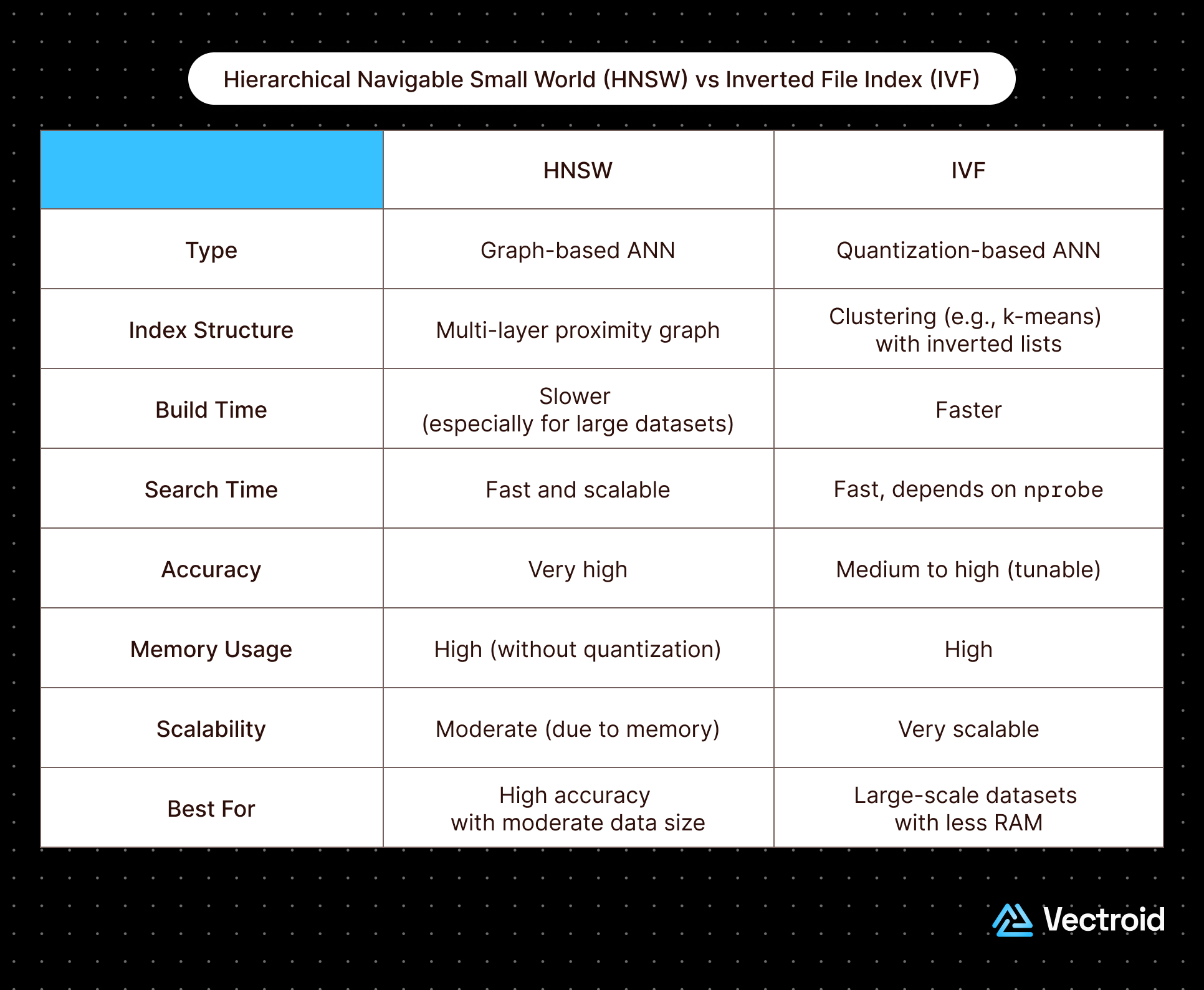
Quick Snapshot: HNSW vs IVF

Before cutting into the details, a quick snapshot of HNSW versus IVF:

What are Hierarchical Navigable Small Worlds (HNSW)?

HNSW is a type of ANN algorithm. HNSW’s origins are in the NSW algorithm, a graph-based approach where any two nodes can be reached with a small numbers of “hops” due to the graph being well-connected and easy to transverse. A crude analogy would be massive Wikipedia—despite being massive, it’s efficient to travel from one article to another through hyperlinks.

To little surprise, the complexity of HNSWs lays in its index construction process. HNSW’s structure is layered NSW graphs. The bottom layer, denoted by $L_0$ contains all of the vectors as nodes; every layer above contains a subset of the vectors on the layer below. Meanwhile, edges connect nearby nodes on the same layer as well as nearby nodes on the layers below.

Construction is iterative; vectors are inserted one-by-one. For each vector, the process follows:

1. Choose highest layer where the vector will appear ($L_{max}$). This is calculated using an exponentially decaying probability distribution so that most points only exist on lower layers. This distribution of nodes across layers is controlled by a normalization parameter, mL, where a higher mL leads to sparser nodes in the upper layers:

$P_{layer} = e^{-layer/mL}$

1. Starting from the vector's $L_{max}$ layer and progressing down to $L_0$:

1. Identify the layer’s entry point(s) aka connections to the layer above (or the global entry points if it’s the topmost layer for the entire graph)
2. Starting from the entry point(s), search for the vector’s nearest neighbors within the layer, perform a greedy search, building up priority queue of closest candidates so far. The max length of this priority queue is controlled by the efConstruction parameter, denoting the maximum number of neighbors that will be evaluated for nearness at each layer. Once the priority queue of candidates reaches length efConstruction, no additional candidate vectors will be considered within the layer. Accordingly, a larger priority queues mean more neighbor candidates and potentially highest quality graph, but indexing will take longer.
3. Create edges between the vector node and the M closest candidate neighbors (first M entries in the priority queue), where M is a parameter which sets the max number of outgoing connections a node can have within a layer
4. Repeat recursively for lower layers, using the closest neighbors from the previous layer to determine the entry points into the current layer

After the HNSW is constructed with all the available vectors, then it could be searched. Searching is more simple. It follow three sub-algorithms:

1. Top Layer Greedy Search. Starting from top layer, perform a greedy search to traverse all nodes in the layer to find the nearest neighbor to the query vector
2. Drop Downs. Drop down to the next layer and repeat the greedy search over the subset of nodes that are connected to the nearest neighbor in the parent layer. This process is repeated until bottom layer is reached.
3. Candidate List Generation. During search, a candidate list (another priority queue) is maintained to store the closest candidate vectors found so far. The max length of this priority queue is controlled by the efSearch parameter. Similar to construction, once the length of the candidate pqueue reaches efSearch, search will terminate and the nearest K neighbors will be returned from the candidate priority queue. A larger efSearch means more vectors will be considered before termination (potentially higher recall) but search will take longer.

What are the benefits of HNSW?

There are a few advantages of HNSWs. The first is that they have excellent performance, boasting high query speeds and high recall. This performance is also generalizable, where it’s maintained over a broad range of dataset sizes and dimensionalities.

Additionally, HNSWs support incremental updates without requiring full re-indexing, which is ideal for workflows where vectors are gradually added to the search engine.

Finally, HNSWs maintain good performance with default parameters without needed tuning. Then, when adding customizability, the HNSW can be optimized for a specific search index by altering the indexing parameters (e.g. mL , efConstruction , M) or search parameters (e.g. efSearch).

Where does HNSW struggle?

One of the biggest challenge with HNSWs is they take a really long time to initially build given the heavily layered approach. Additionally, inserting new vectors, while not requiring a full re-index, are slower than other ANN algorithms.

Additionally, HNSWs are memory intensive, requiring more space than other ANN algorithms. However, memory usage can be minimized by reducing the number of layers or compressing vectors (for example, using binary quantization where values are snapped to approximations).

From a purely developer point-of-view, HNSWs are also naturally complex to implement given the involvement of the algorithm. However, most developers will choose to use a managed HNSW implemented by a database, not a homegrown solution.What is IVF (Inverted File Index)?

IVF is another variant of ANNs that rely on clustering to partition the vector space into distinct regions (or buckets or cells). This approach focuses the search effort on only relevant regions to reduce the number of distance calculations needed.

To construct an index:

1. A clustering algorithm (such as k-means) is performed to identify nlist cluster “centroids”, which is the cluster’s central point / arithmetic mean / “prototypical” data point. nlist is a parameter defines the number of clusters to be created from the dataset; the effectiveness of IVF strongly relies on the performance of the clustering algorithm. A good algorithm should partition the search space into cohesive, distinct clusters.
2. Each vector in the search space is assigned to its nearest centroid; each of the nlist centroids then has its own “inverted list” of assigned vectors (aka a “bucket” or “cell”). These inverted lists have various storage options. Sometimes, they may contain the full vectors themselves (i.e. “IVFFlat”), which is very accurate but can be memory intensive and slow. More commonly, IVF implementations populate each inverted list with a compressed representation of each vector, often using Product Quantization. This method is called ”IVFPQ” or “IVFADC” for “Asymmetric Distance Calculation”, since the original search vector is being compared to an approximate distance to the compressed original. This effectively trades off accuracy for speed / memory footprint. In some cases, the original search vector is also compressed (this is called IVFSDC for “Symmetric Distance Calculation”), which is even faster but less accurate.

Once the index is constructed, search is relatively simple. This is a two-step process:

1. A search query is compared to all k centroids to identify the nprobe nearest centroids. The nprobe parameter is the max number of centroids whose list members will be considered for more precise search calculations. Accordingly, a higher nprobe means more candidates will be considered and potentially better chances of finding true nearest neighbors, but search will take longer.
2. Then, a more precise search calculation is then conducted over the inverted lists of the top nprobe centroids (comparing the query vector to each candidate vector in the list). After the precise search is complete, the top K nearest vectors are returned.

What are advantages of IVF?

An IVF variant of ANN is highly performant when data has natural clusters. In other words, if the clustering algorithm is effective at partitioning the search space, then IVF is incredibly fast. This makes IVF’s performance a data-dependent metric.

Additionally, IVF is highly scalable and very memory efficient, especially when vectors are compressed. When optimized, IVF has a smaller memory footprint than HNSW. This makes it a particularly good choice for large datasets.

IVF is also very fast to update in real time, where inserting new vectors into the data space is quick. However, the data distribution may change the effectiveness of cluster partitioning.

Finally, from a developer point-of-view, IVF is one of the simplest ANN algorithms to implement. Creating inverted lists is largely abstracted away by the clustering algorithm of choice.

Where are disadvantages of IVF?

One tricky aspect of IVF is its data dependence. Not all datasets are well represented by clustering algorithms, and badly clustered data will result in inaccurate and/or slow queries.

IVF also struggles with high dimensionality datasets, something known as the “curse of dimensionality” where performance sharply degrades. In particular, the performance and effectiveness of algorithms in high dimension spaces suffers whenever data points are spread out and sparse as it’s harder to create good clusters. This also makes IVF a poor candidate for dynamic datasets where the cluster quality degrades with time due to drifts in data distribution.

Final Thoughts: HNSW vs IVF

HNSW is a better choice than IVF when:

You want fast query speeds AND high recall. HNSW generally outperforms IVF in both departments across a wide range of data scales and dimensionality.

Your dataset has high dimensionality. HNSW tolerates high dimensionality much better than IVF since a well connected graph is a better representation of true connectivity than a poorly defined cluster.

Your dataset is subject to drifts in data distribution. Without reindixing, IVF’s cluster efficiency is reliant on the incoming data naturally sorting itself into appropriate clusters — if that cant be guaranteed, you may see degraded accuracy and query perf. HNSW in contrast handles data drifts very well!

You want good performance without heavy tuning. IVF recall is sensitive to choices like nlist and nprobe , which often require workload-specific tuning. HNSW is less finicky and usually “just works” with reasonable defaults.

Use IVF over HNSW if:

Memory efficiency is your priority. IVF is generally requires less memory than HNSW since it doesnt have to store graph edges which are complex, dense data structures. IVF also integrates naturally with PQ, which can drastically shrink memory footprint and improve cache efficiency. HNSW can use PQ too, but IVF+PQ is the more standard combo.

Your dataset is naturally and predictably clustered. IVF has good accuracy and recall when the underlying data is well represented by the clusters and updates maintain the initial data distribution. HNSW will represent this data well too, but it may be overkill relative to IVF in terms of memory usage.

You’re frequently running batch queries. IVF often performs better in batched or GPU-accelerated scenarios since probing clusters can be parallelized more easily than traversing a graph.

You want to keep things simple. IVF is much simpler to reason about and set up than HNSW. if you cant commit to the complexity of building an maintaining an HNSW implementation, IVF is more straightforward. for example, if your dataset receives frequent updates and you want new data to be immediately queryable, you can see faster insertion times with IVF versus HNSW out of the box. Real time querability with HNSW is still achievable but it requires more thought and development effort (for example, Vectroid accomplished this by implementing secondary instantaneous datastore for recent data while new indexes run)