HNSW vs DiskANN: comparing the leading ANN algorithms

Vector search is core building block for applications like semantic search, recommendation, and retrieval-augmented generation (RAG). At scale, finding nearest neighbors quickly and cost-effectively is a hard problem, hence the development of Approximate Nearest Neighbor (ANN) algorithms.

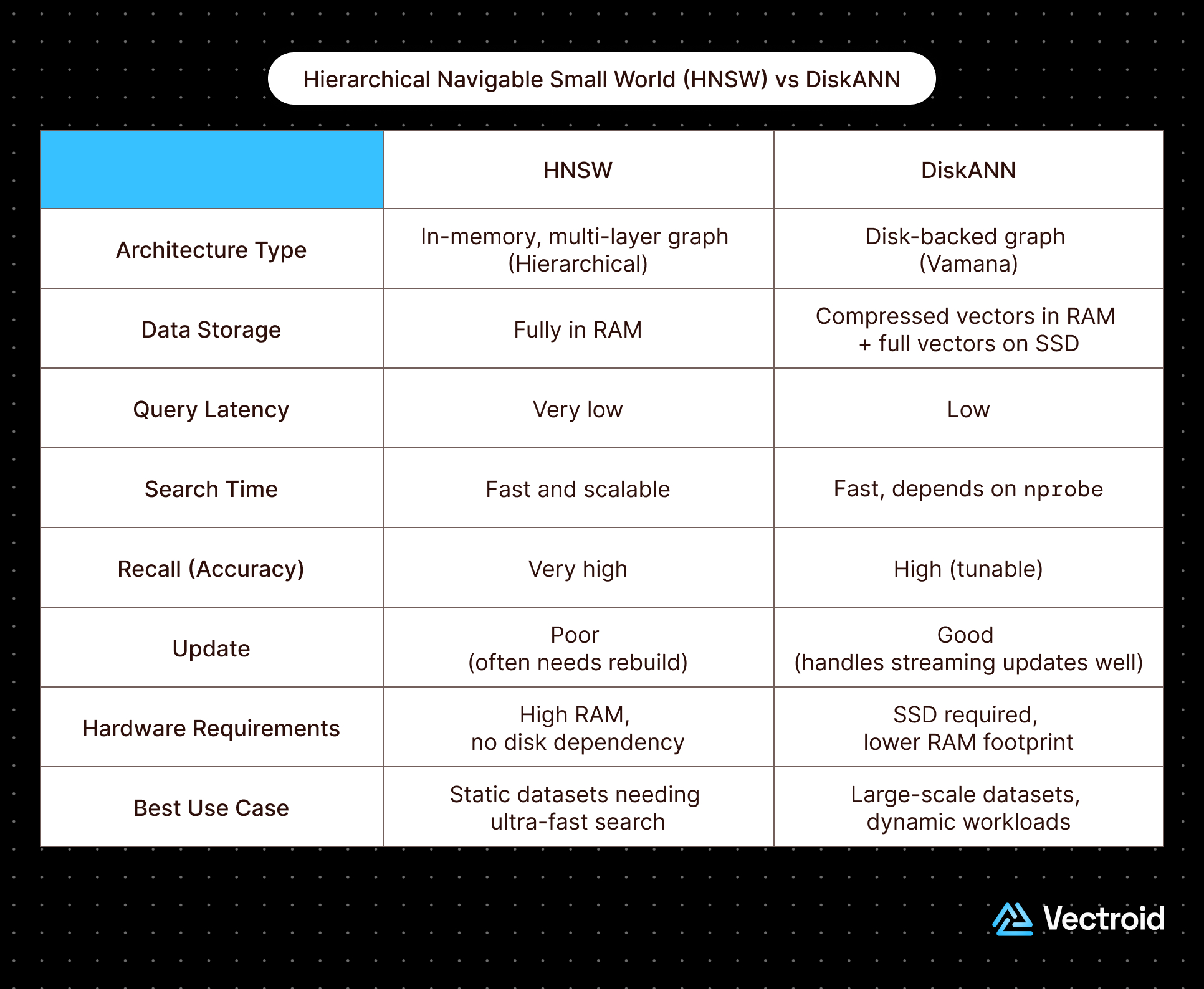
There are two leading ANN implementations for vector search:

HNSW (Hierarchical Navigable Small World graphs), which is the most widely adopted in-memory graph-based ANN index
DiskANN (Disk-Accelerated Nearest Neighbor search), a newer graph-based method from Microsoft designed to extend ANN to billion-scale datasets using SSDs

In this article, we’ll explain how HNSW and DiskANN works, compare their strengths and tradeoffs, and provide guidance on when to choose one over the other.

What are Hierarchical Navigable Small Worlds (HNSWs)

HNSW is a graph-based ANN algorithm designed for high recall and low latency in-memory vector search. It has become one of the most popular ANN algorithms due to its robust and consistent performance across many shapes and dimensions of datasets.

At its core, HNSW uses a multi-layer graph structure based on small-world networks. The upper layers contain long-range “express” links that allow rapid traversal of the space, while the lower layers contain dense local connections that refine the nearest neighbor search.

HNSW’s Index

Typically, the entire HNSW index resides in RAM to enable low-latency lookups. In many implementations, the index stores full-precision vectors, though some implementations compress vectors with binary or product quantization to reduce memory usage (at the cost of some recall accuracy).

The index is built incrementally as new vectors are added. For each new vector, a maximum layer height is assigned, sampled from an exponential distribution (similar to how skip lists probabilistically assign levels). Higher layers are sparse and act as shortcuts, while the lower layers are denser. In most implementations, the base layer includes every data point. Insertion proceeds top-down, beginning at the highest level. Starting from a global or random entry point, the algorithm performs a greedy search to find candidate neighbors. Once identified, the new vector connects to its M nearest neighbors, where M controls graph connectivity.

HNSW Pruning

To prevent redundant edges and encourage diversity, HNSW applies a pruning strategy—similar in behavior to DiskANN’s RobustPrune—that removes neighbors too close in distance and direction to existing ones. The process then drops down one layer and repeats, using the entry point from the previous layer until reaching the base.

Searching HNSWs

The search process starts at the highest layer, where the graph is sparse and dominated by long-range links. From a designated or random entry point, the algorithm performs a greedy search, always moving to the neighbor closest to the query vector until no closer neighbor remains. It then descends one layer, using the last candidate as the new entry point and repeating.

Once reaching the base layer, instead of a pure greedy search, HNSW employs a beam search (best-first search) to balance exploration and exploitation. This search maintains a candidate list (of size efSearch) as a priority queue, expanding nodes by checking neighbors and keeping only the closest candidates. Once the exit condition is met—such as stabilization of the list or retrieval of efSearch entries—the top k nearest neighbors are returned.

Benefits of HNSWs

HNSW shines in several areas:

It delivers low latency and high recall since the index is memory-resident and avoids disk I/O, enabling sub-millisecond queries.
Its incremental construction makes index build times fast and allows new vectors to be added without requiring a full rebuild.
It is also simple and mature, with widely documented parameters and predictable behavior, often working well without extensive tuning.

For small to medium datasets that fit in RAM, HNSW provides strong baseline performance, making it the de facto standard in many libraries.

Drawbacks of HNSWs

However, HNSW has its limitations. It consumes large amounts of memory since the full graph—including all vector data and edges—must reside in RAM. This becomes prohibitively expensive at billion vector scale. Its scalability is also limited because it is not designed for disk-based operation; extending it beyond RAM requires hybrid systems that diminish its performance. Deletions are also inefficient as they require tombstoning or a full rebuild.

What is DiskANN?

DiskANN is a graph-based ANN algorithm developed by Microsoft, designed for highly scalable and cost-effective search over massive vector datasets. It achieves scalability by leveraging high-speed SSD storage, reducing reliance on expensive RAM.

DiskANN’s indexing

DiskANN’s core data structure is based on the Vamana graph algorithm, a strategy optimized for efficient routing of queries via greedy search. DiskANN differs from Vamana by employing greedy search and robust pruning during construction to optimize index building and querying. Most of the index, including uncompressed vectors, is stored on SSDs, while compressed versions of vectors are held in RAM to guide searches and minimize disk reads.

Index construction is time-consuming because the data structure prioritizes fast querying over fast indexing. It begins with a random graph, assigning each node a fixed maximum number of outgoing edges (R). The graph is then iteratively optimized. For each node, approximate neighbors are identified via greedy search simulations, and the node’s neighborhood is pruned and optimized.

RobustPrune

DiskANN uses the RobustPrune heuristic to maintain diversity: it evaluates candidate neighbors by both distance and angular diversity relative to existing neighbors, pruning redundant edges. Iterations continue until the graph stabilizes or a maximum iteration count is reached.

To perform RobustPrune, there are a few steps:

Sort the candidate neighbors of p
Starting from the nearest candidate (p’), iterate through the candidates to determine whether or not to add it as a neighbor. This is done by adding a potential edge between p and p’. Then, if the edge is too close in distance and direction to p (determined by a tunable parameter a), prune it.
Once R neighbors have been added, stop iterating.

Searching DiskANN

The search process starts by querying the compressed in-memory graph to find top candidates. These candidates’ full-precision vectors are then fetched from SSD in batched reads, made possible by the graph’s contiguous on-disk layout that clusters related vectors together. The retrieved vectors are compared against the query and re-ranked to produce accurate results.Benefits of DiskANN

DiskANN excels at cost-effective scalability:

By optimizing for SSD usage, it minimizes RAM requirements and reduces hardware costs, making it ideal for massive datasets.
It achieves high accuracy and low latency at scale by combining in-memory compressed searches with batched SSD reads.
One variant known as FreshDiskANN supports real-time updates and hybrid vector-plus-filtered search, addressing long-standing limitations in some vector databases.

Drawbacks of DiskANN

On the other hand, DiskANN suffers from slow build times, as constructing and optimizing the Vamana graph is computationally heavy. Its performance is also tied to SSD throughput and latency, which may degrade in constrained environments.

While updates are supported, they remain more expensive than with in-memory structures like HNSW. Finally, DiskANN’s implementation and tuning are complex, involving multiple moving parts, pruning heuristics, and storage optimizations.

Choosing Between DiskANN and HNSW

both HNSW and DiskANN utilize proximity related graphs, but they have different approaches to graph construction and traversal which means they are optimized for different application priorities.Use HNSW over DiskANN if…

Your dataset can fit comfortably (and affordably) in memory. If your vectors fit in RAM, HNSW will be simpler, faster to build, and cheaper to operate since it avoids disk I/O altogether

You have strict query latency requirements. HNSW is purely in-memory, so it will always have an advantage in query speed over DiskANN since it is able to avoid any time-consuming disk I/O.

You want a simpler implementation. HNSW is widely supported in most open-source vector libraries and managed services, and it has and well-understood tuning knobs.

You want to avoid complex fine tuning. HNSW typically works well with default settings, while DiskANN may require more complicated refinement and experimentation with parameter tuning (graph out-degree, SSD layout, pruning heuristics).

Use DiskANN over HNSW if…

Your dataset is too big to fit in memory. When storing hundreds of millions or billions of vectors, HNSW’s memory requirements become cost-prohibitive, while DiskANN leverages SSDs to scale cost-effectively beyond RAM limits

You want to reduce infrastructure costs. SSDs are far cheaper per GB than RAM, so DiskANN can deliver high recall and low latency at a fraction of the memory cost for very large datasets

You need filtered or hybrid search at scale. DiskANN’s newer versions natively support combining vector similarity with structured filters. HNSW-based systems may struggle to return correct or complete results in these scenarios because if filtered-out nodes happen to be on the traversal path (neighbors of the query or key graph hubs), they effectively “block” access to other valid nodes

You need ongoing real-time updates at massive scale. FreshDiskANN supports inserts, deletes, and updates without requiring full index rebuilds, making it better suited for continuously evolving datasets (ideal for search engines, recommendation feeds, etc.)